“I want friends to motion such matter.”
Up until now, the image has remained in a fixed position, in this chapter we take a look at how we can start repositioning samples.
Affine transformations are transformations to an image that preserves colinearity, all points on a line remains on a line after transformation. Usually affine transformations are expressed as an matrices, in this text to keep the math level down, I will use geometry and vectors instead.
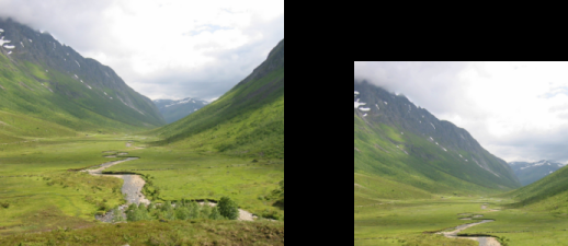
Translation can be described as moving the image, e.g. move all the contents of the image 50pixels to the right and 50pixels down.
Instead of traversing the original image, and placing the pixels in their new location we calculate which point in the source image ends up at the coordinate calculated.
Figure 6.1. translation
function translate(dx,dy)
  for y=0, height-1 do
    for x=0, width-1 do
      -- calculate the source coordinates (u,v)
      u = x-dx
      v = y-dy

      r,g,b=get_rgba(u,v)
      set_rgb(x,y,r,g,b)
    end
    progress (y/height)
  end
  flush()
end

translate(width*0.25,height*0.25)
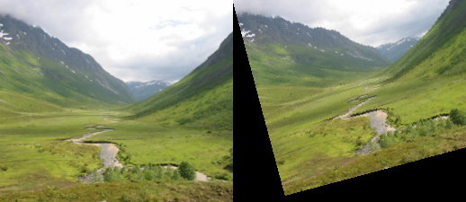
Rotation is implemented by rotating the unit vectors of the coordinate system, and from the unit vectors calculate the new positions of a given input coordinate, to make the transformation happen in reverse it is enough to negate the angle being passed to our function.
Figure 6.2. rotation
function rotate(angle)
  for y=0, height-1 do
    for x=0, width-1 do
      -- calculate the source coordinates (u,v)
      u = x * math.cos(-angle) + y * math.sin(-angle)
      v = y * math.cos(-angle) - x * math.sin(-angle)

      r,g,b = get_rgba(u,v)
      set_rgb(x,y,r,g,b)
    end
    progress (y/height)
  end
  flush()
end

rotate(math.rad(15))
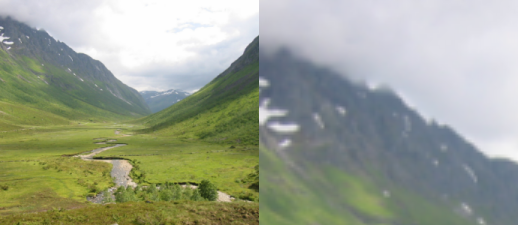
Scaling an image is a matter of scaling both the x and y axes according to a given scale factor when retrieving sample values.
Figure 6.3. scaling

function scale(ratio)
  for y=0, height-1 do
    for x=0, width-1 do
      -- calculate the source coordinates (u,v)
      u = x * (1.0/ratio)
      v = y * (1.0/ratio)

      r,g,b = get_rgba(u,v)
      set_rgb(x,y,r,g,b)
    end
    progress (y/height)
  end
  flush()
end

scale(3)
Perspective transformations are useful for texture mapping, texture mapping is outside the scope of this text. Affine transformations are a subset of perspective transformations.
To be able to do texturemapping for use in realtime 3d graphics, the algorithm is usually combined with a routine that only paints values within the polygon defined, such a routine is called a polyfiller.
When doing rotation as well as scaling, the coordinates we end up getting pixel values from are not neccesary integer coordinates. When enlarging this problem is especially apparent in Figure 6.3, “scaling” the problem is quite apparent we have "enlarged" each sample (pixel) to cover a larger area, this results in blocky artifacts within the image.
A more correct approach is to make an eduacted guess about the missing value at the sampling coordinates, this means attempting to get the results we would have gotten by sampling that coordinate in the original continous analog image plane.
The method used in the affine samples above is called "nearest neighbour", getting the closest corresponding pixel in the source image.
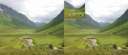
Bilinear sampling makes the assumption that values in the image changes continously.
Figure 6.4. bilinear
function get_rgb_bilinear (x,y)
  local x0,y0 -- integer coordinates
  local dx,dy -- offset from coordinates
  local r0,g0,b0, r1,g1,b1, r2,g2,b2, r3,g3,b3
  local r,g,b

  x0=math.floor(x)
  y0=math.floor(y)
  dx=x-x0
  dy=y-y0

  r0,g0,b0 = get_rgb (x0  ,y0  )
  r1,g1,b1 = get_rgb (x0+1,y0  )
  r2,g2,b2 = get_rgb (x0+1,y0+1)
  r3,g3,b3 = get_rgb (x0  ,y0+1)

  r = lerp (lerp (r0, r1, dx), lerp (r3, r2, dx), dy)
  g = lerp (lerp (g0, g1, dx), lerp (g3, g2, dx), dy)
  b = lerp (lerp (b0, b1, dx), lerp (b3, b2, dx), dy)

  return r,g,b
end

function scale(ratio)
  for y=0, height-1 do
    for x=0, width-1 do
      -- calculate the source coordinates (u,v)
      u = x * (1.0/ratio)
      v = y * (1.0/ratio)
      r,g,b=get_rgb_bilinear(u,v)
      set_rgb(x,y,r,g,b)
    end
    progress (y/height)
  end
  flush()
end

function lerp(v1,v2,ratio)
   return v1*(1-ratio)+v2*ratio;
end
-- LERP
-- /lerp/, vi.,n.
--
-- Quasi-acronym for Linear Interpolation, used as a verb or noun for
-- the operation. "Bresenham's algorithm lerps incrementally between the
-- two endpoints of the line." (From Jargon File (4.4.4, 14 Aug 2003)
scale(3)
Figure 6.5. bicubic

function get_rgb_cubic_row(x,y,offset)
  local r0,g0,b0, r1,g1,b1, r2,g2,b2, r3,g3,b3
  r0,g0,b0 = get_rgb(x,y)
  r1,g1,b1 = get_rgb(x+1,y)
  r2,g2,b2 = get_rgb(x+2,y)
  r3,g3,b3 = get_rgb(x+3,y)
  return cubic(offset,r0,r1,r2,r3), cubic(offset,g0,g1,g2,g3), cubic(offset,b0,b1,b2,b3)
end

function get_rgb_bicubic (x,y)
  local xi,yi -- integer coordinates
  local dx,dy -- offset from coordinates
  local r,g,b

  xi=math.floor(x)
  yi=math.floor(y)
  dx=x-xi
  dy=y-yi

  r0,g0,b0 = get_rgb_cubic_row(xi-1,yi-1,dx)
  r1,g1,b1 = get_rgb_cubic_row(xi-1,yi,  dx)
  r2,g2,b2 = get_rgb_cubic_row(xi-1,yi+1,dx)
  r3,g3,b3 = get_rgb_cubic_row(xi-1,yi+2,dx)

  return cubic(dy,r0,r1,r2,r3),
         cubic(dy,g0,g1,g2,g3),
         cubic(dy,b0,b1,b2,b3)
end

function scale(ratio)
  for y=0, height-1 do
    for x=0, width-1 do
      -- calculate the source coordinates (u,v)
      u = x * (1.0/ratio)
      v = y * (1.0/ratio)
      r,g,b=get_rgb_bicubic(u,v)
      set_rgb(x,y,r,g,b)
    end
    progress (y/height)
  end
  flush()
end

function cubic(offset,v0,v1,v2,v3)
  -- offset is the offset of the sampled value between v1 and v2
   return   (((( -7 * v0 + 21 * v1 - 21 * v2 + 7 * v3 ) * offset +
               ( 15 * v0 - 36 * v1 + 27 * v2 - 6 * v3 ) ) * offset +
               ( -9 * v0 + 9 * v2 ) ) * offset + (v0 + 16 * v1 + v2) ) / 18.0;
end

scale(3)
When scaling an image down the output contains fewer pixels (sample points) than the input. We are not guessing the value of in-between locations, but combining multiple input pixels to a single output pixel.
One way of doing this is to use a box filter and calculate a weighted average of the contribution of all pixel values.
Figure 6.6. box decimate
function get_rgb_box(x0,y0,x1,y1)
  local area=0 -- total area accumulated in pixels
  local rsum,gsum,bsum = 0,0,0
  local x,y
  local xsize, ysize

  for y=math.floor(y0),math.ceil(y1) do
    ysize = 1.0
    if y<y0 then
      size = size * (1.0-(y0-y))
    end
    if y>y1 then
      size = size * (1.0-(y-y1))
    end
    for x=math.floor(x0),math.ceil(x1) do
      size = ysize
      r,g,b = get_rgb(x,y)
      if x<x0 then
        size = size * (1.0-(x0-x))
      end
      if x>x1 then
        size = size * (1.0-(x-x1))
      end
      rsum,gsum,bsum = rsum + r*size, gsum + g*size, bsum + b*size
      area = area+size
    end
  end

  return rsum/area, gsum/area, bsum/area
end

function scale(ratio)
  for y=0, (height*ratio)-1 do
    for x=0, (width*ratio)-1 do
      u0 = x * (1.0/ratio)
      v0 = y * (1.0/ratio)
      u1 = (x+1) * (1.0/ratio)
      v1 = (y+1) * (1.0/ratio)
      r,g,b=get_rgb_box(u0,v0,u1,v1)
      set_rgb(x,y,r,g,b)
    end
    progress (y/(height*ratio))
  end
  flush()
end

scale(0.33)
With OpenGL and other realtime 3d engines it is common to use mipmaps to increase processing speed and the quality of the resampled texture.
A mipmap is a collection of images of prescaled sizes. The prescaled sizes are 1.0×image dimensions, 0.5×image dimensions, 0.25×image dimensions, 0.125×image dimensions etc.
When retrieving a sample value a bilinear interpolation would be performed at both the version of the image larger than the scaling ratio as well as the image smaller than the scaling ratio. After that a linear interpolation is performed on the two resulting values based on which of the two versions most closely matches the target resolution.
Using The GIMP open a test image, create a duplicate of the original image. (Image/Duplicate). Scale the duplicate image to 25% size (Image/Scale). Scale the duplicate image up 400%. Copy the newly scaled image as a layer on top of the original image. (Ctrl+C, change image Ctrl+V), and press the new layer button when the original image is active. Set the mode of the top layer to difference, Flatten the image (Image/Flatten Image), and automatically stretch the contrast of the image. (Layer/Colors/Auto/Stretch Contrast).
Do this for nearest neighbour, bilienar and bicubic interpolation and compare the results.
Read Appendix A, Assignment, spring 2007 and perhaps make initial attempts at demosaicing the Bayer pattern.