“If thence he 'scappe, into whatever world, Or unknown region.”
In Chapter 4, Point operations we looked at operations that calculated the new sample values of a pixel based on the value of the original pixel alone. In this chapter we look at the extension of that concept, operations that take their input from a local neighbourhood of the original pixel.
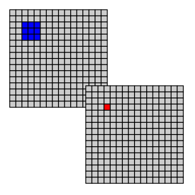
We can sample with different input windows the most common are a square or circle centered on the pixel as shown in Figure 5.1, “Sliding window”.
Figure 5.1. Sliding window
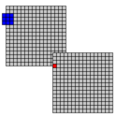
When sampling a local area around a pixel, we need to decide what to do when part of the sampling window is outside the source image. The common way to provide a "fake" value for data outside the image are:
- Make them transparent.
- Give them a color (for instance black).
- Nearest valid pixel.
- Mirror the image over the edge.
- Wrap to other side of image.
In gluas the global variable edge_duplicate can be set to 1, this makes gluas return the nearest valid pixel instead of transparent/black.
Figure 5.2. Over the edge
A special group of operations are the kernel filters, which use a table of numbers (a matrix) as input. The matrix gives us the weight to be given each input sample. The matrix for a kernel filter is always square and the number of rows/columns are odd. Many image filters can be expressed as convolution filters some are listed in the sourcelisting in Figure 5.3, “convolve”.
Each sample in the sampling window is weighted with the corresponding weight in the convolution matrix. The resulting sum is divided by the divisor (for most operations this is assumed to be the sum of the weights in the matrix). And finally an optional offset might be added to the result.
Figure 5.3. convolve
-- 3x3 convolution filter
edge_duplicate=1;
function convolve_get_value (x,y, kernel, divisor, offset)
local i, j, sum
sum_r = 0
sum_g = 0
sum_b = 0
for i=-1,1 do
for j=-1,1 do
r,g,b = get_rgb (x+i, y+j)
sum_r = sum_r + kernel[j+2][i+2] * r
sum_g = sum_g + kernel[j+2][i+2] * g
sum_b = sum_b + kernel[j+2][i+2] * b
end
end
return sum_r/divisor + offset, sum_g/divisor+offset, sum_b/divisor+offset
end
function convolve_value(kernel, divisor, offset)
for y=0, height-1 do
for x=0, width-1 do
r,g,b = convolve_get_value (x,y, kernel, divisor, offset)
set_rgb (x,y, r,g,b)
end
progress (y/height)
end
flush ()
end
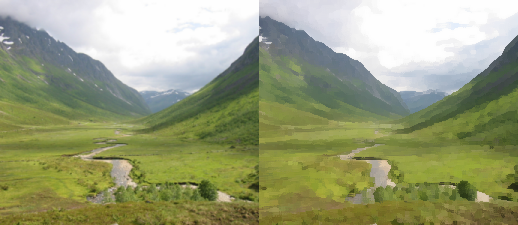
function emboss()
kernel = { { -2, -1, 0},
{ -1, 1, 1},
{ 0, 1, 2}}
divisor = 1
offset = 0
convolve_value(kernel, divisor, offset)
end
function sharpen()
kernel = { { -1, -1, -1},
{ -1, 9, -1},
{ -1, -1, -1}}
convolve_value(kernel, 1, 0)
end
function sobel_emboss()
kernel = { { -1, -2, -1},
{ 0, 0, 0},
{ 1, 2, 1}}
convolve_value(kernel, 1, 0.5)
end
function box_blur()
kernel = { { 1, 1, 1},
{ 1, 1, 1},
{ 1, 1, 1}}
convolve_value(kernel, 9, 0)
end
sharpen ()
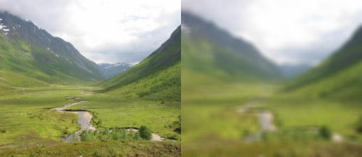
A convolution matrix with all weights set to 1.0 is a blur, blurring is an operation that is often performed and can be implemented programmatically faster than the general convolution. A blur can be seen as the average of an area, or a resampling which we'll return to in a later chapter.
Figure 5.4. blur
-- a box blur filter implemented in lua

edge_duplicate = 1;

function blur_slow_get_rgba(sample_x, sample_y, radius)
   local x,y
   local rsum,gsum,bsum,asum=0,0,0,0
   local count=0

   for x=sample_x-radius, sample_x+radius do
     for y=sample_y-radius, sample_y+radius do

       local r,g,b,a= get_rgba(x,y)

       rsum, gsum, bsum, asum = rsum+r, gsum+g, bsum+b, asum+a

       count=count+1
     end
   end
   return rsum/count, gsum/count, bsum/count, asum/count
end

function blur_slow(radius)
    local x,y


    for y = 0, height-1 do
        for x = 0, width-1 do
           set_rgba (x,y, blur_slow_get_rgba (x,y,radius))
        end
        progress (y/height)
    end
    flush ()
end


-- seperation into two passes, greatly increases the speed of this
-- filter

function blur_h_get_rgba(sample_x, sample_y, radius)
   local x,y
   local rsum,gsum,bsum,asum=0,0,0,0
   local count=0

   y=sample_y
   for x=sample_x-radius, sample_x+radius do
       local r,g,b,a= get_rgba(x,y)

       rsum, gsum, bsum, asum = rsum+r, gsum+g, bsum+b, asum+a

       count=count+1
   end
   return rsum/count, gsum/count, bsum/count, asum/count
end

function blur_v(radius)
    for y = 0, height-1 do
        for x = 0, width-1 do
           set_rgba (x,y, blur_v_get_rgba(x,y,radius))
        end
        progress(y/height)
    end
    flush()
end

function blur_v_get_rgba(sample_x, sample_y, radius)
   local x,y
   local rsum,gsum,bsum,asum=0,0,0,0
   local count=0

   x=sample_x
   for y=sample_y-radius, sample_y+radius do
       local r,g,b,a= get_rgba(x,y)

       rsum, gsum, bsum, asum = rsum+r, gsum+g, bsum+b, asum+a

       count=count+1
   end
   return rsum/count, gsum/count, bsum/count, asum/count
end

function blur_h(radius)
    for y = 0, height-1 do
        for x = 0, width-1 do
           set_rgba (x,y, blur_h_get_rgba(x,y,radius))
        end
        progress(y/height)
    end
    flush()
end

function blur_fast(radius)
  blur_v(radius)
  blur_h(radius)
end

blur_fast(4)
A better looking blur is achieved by setting the weights to a gaussian distribution around the active pixel.
A gaussian blur works by weighting the input pixels near the center of ther sampling window higher than the input pixels further away.
One way to approximate a small gaussian blur, is to set the center pixel in a 3×3 matrix to 2, while the surrounding are set to 1, and set the weight to 10.
A blur is a time consuming operation especially if the radius is large. A way to optimize a blur is to observe that first blurring horizontally and then vertically gives the same result as doing both at the same time. This has been done to the blur_fast in Figure 5.4, “blur” and can also be done for gaussian blurs.
Edge preserving smoothing filters are useful for automated feature detection or even just for artistic effects.
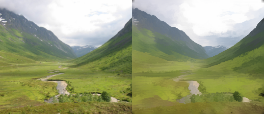
The kuwahara filter is an edge preserving blur filter. It works by calculating the mean and variance for four subquadrants, and chooses the mean value for the region with the smallest variance.
Figure 5.5. kuwahara
-- Kuwahara filter
--
--
-- Performs the Kuwahara Filter. This filter is an edge-preserving filter.
--
--
-- ( a  a  ab   b  b)
-- ( a  a  ab   b  b)
-- (ac ac abcd bd bd)
-- ( c  c  cd   d  d)
-- ( c  c  cd   d  d)
--
-- In each of the four regions (a, b, c, d), the mean brightness and the variance are calculated. The
-- output value of the center pixel (abcd) in the window is the mean value of that region that has the
-- smallest variance.
--
-- description copied from http://www.incx.nec.co.jp/imap-vision/library/wouter/kuwahara.html
--
-- implemented by Øyvind Kolås <oeyvindk@hig.no> 2004


-- the sampling window is:  width=size*2+1  height=size*2+1

size = 4

edge_duplicate = 1;

-- local function to get the mean value, and
-- variance from the rectangular area specified
function mean_and_variance (x0,y0,x1,y1)
 local variance
 local mean

 local min         = 1.0
 local max         = 0.0
 local accumulated = 0
 local count       = 0

 local x, y

 for y=y0,y1 do
   for x=x0,x1 do
     local v = get_value(x,y)

     accumulated   = accumulated + v
     count         = count + 1

     if v<min then min = v end
     if v>max then max = v end

    end
  end

  variance = max-min
  mean     = accumulated /count

  return mean, variance
end

-- local function to get the mean value, and
-- variance from the rectangular area specified
function rgb_mean_and_variance (x0,y0,x1,y1)
 local variance
 local mean
 local r_mean
 local g_mean
 local b_mean

 local min           = 1.0
 local max           = 0.0
 local accumulated_r = 0
 local accumulated_g = 0
 local accumulated_b = 0
 local count         = 0

 local x, y

 for y=y0,y1 do
   for x=x0,x1 do
     local v     = get_value(x,y)
     local r,g,b = get_rgb (x,y)

     accumulated_r   = accumulated_r + r
     accumulated_g   = accumulated_g + g
     accumulated_b   = accumulated_b + b
     count         = count + 1

     if v<min then min = v end
     if v>max then max = v end

    end
  end

  variance = max-min
  mean_r   = accumulated_r /count
  mean_g   = accumulated_g /count
  mean_b   = accumulated_b /count

  return mean_r, mean_g, mean_b, variance
end

-- return the kuwahara computed value
function kuwahara(x, y, size)
  local best_mean     = 1.0
  local best_variance = 1.0

  local mean, variance

  mean, variance = mean_and_variance (x-size, y-size, x, y)

  if variance < best_variance then
    best_mean     = mean
    best_variance = variance
  end

  mean, variance = mean_and_variance (x, y-size, x+size,y)

  if variance < best_variance then
    best_mean     = mean
    best_variance = variance
  end

  mean, variance = mean_and_variance (x, y, x+size, y+size)

  if variance < best_variance then
    best_mean     = mean
    best_variance = variance
  end

  mean, variance = mean_and_variance (x-size, y, x,y+size)

  if variance < best_variance then
    best_mean     = mean
    best_variance = variance
  end

  return best_mean
end


-- return the kuwahara computed value
function rgb_kuwahara(x, y, size)
  local best_r, best_g, best_b
  local best_variance = 1.0

  local r,g,b, variance

  r,g,b, variance = rgb_mean_and_variance (x-size, y-size, x, y)

  if variance < best_variance then
    best_r, best_g, best_b = r, g, b

    best_variance = variance
  end

  r,g,b, variance = rgb_mean_and_variance (x, y-size, x+size,y)

  if variance < best_variance then
    best_r, best_g, best_b = r, g, b
    best_variance = variance
  end

  r,g,b, variance = rgb_mean_and_variance (x, y, x+size, y+size)

  if variance < best_variance then
    best_r, best_g, best_b = r, g, b
    best_variance = variance
  end

  r,g,b, variance = rgb_mean_and_variance (x-size, y, x,y+size)

  if variance < best_variance then
    best_r, best_g, best_b = r, g, b
    best_variance = variance
  end

  return best_r, best_g, best_b
end

function kuwahara(radius)
  for y=0, height-1 do
    for x=0, width-1 do
      r,g,b = rgb_kuwahara (x,y, radius)
      set_rgb (x,y, r,g,b)
    end
    progress (y/height)
  end
end

kuwahara(2)
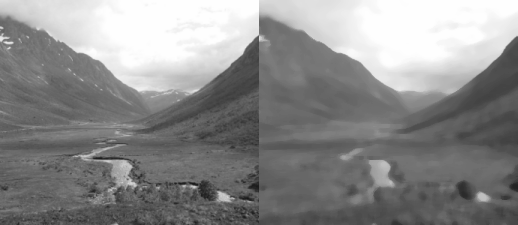
An improvement over the kuwahara filter is the symmetric nearest neighbour filter that compares symmetric pairs/quadruples of pixels with the center pixel and only takes into account the one from this set which is closest in value to the center pixel.
Figure 5.6. snn
-- Symmetric Nearest Neighbour as described by Hardwood et al in Pattern
-- recognition letters 6 (1987) pp155-162.

function snn(radius)
local x,y
for y=0, height-1 do
	for x=0, width-1 do
	    local sum=0.0
	    local count=0.0
	    local u,v

	    local valueC = get_value (x,y)

	    for v=-radius,radius do
	      for u=-radius,radius do
	         local valueA = get_value (x+u,y+v)
	         local valueB = get_value (x-u,y-v)

	         if (math.abs(valueC-valueA) <
	             math.abs(valueC-valueB)) then
               sum = sum + valueA
	         else
               sum = sum + valueB
	         end
	         count = count + 1
	      end
	    end
		set_value (x,y, sum/count)
	end
	progress (y/height)
end
flush()
end

-- snn(6)

-- and a color version operating in CIE Lab

function deltaE(l1,a1,b1,l2,a2,b2)
  return math.sqrt( (l1-l2)*(l1-l2) + (a1-a2)*(a1-a2) + (b1-b2)*(b1-b2))
end

function snn_color(radius)
local x,y
for y=0, height-1 do
	for x=0, width-1 do
	    local sumL=0.0
	    local suma=0.0
	    local sumb=0.0
	    local count=0.0
	    local u,v

	    local lc,ac,bc = get_lab (x,y)

	    for v=-radius,radius do
	      for u=-radius,radius do
			 local l1,a1,b1 = get_lab (x+u,y+v)
	         local l2,a2,b2 = get_lab (x-u,y-v)

	         if (deltaE(lc,ac,bc,l1,a1,b1) <
	             deltaE(lc,ac,bc,l2,a2,b2)) then
               sumL = sumL + l1
               suma = suma + a1
               sumb = sumb + b1
	         else
	           sumL = sumL + l2
               suma = suma + a2
               sumb = sumb + b2
	         end
	         count = count + 1
	      end
	    end
		set_lab (x,y, sumL/count, suma/count, sumb/count)
	end
	progress (y/height)
end
flush()
end
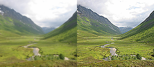
snn_color(6)Rank filters operate statistically on the neighbourhood of a pixel. The tree most common rank filters are median, minimum, maximum.
The median filter sorts the sample values in theneighbourhood, and then picks the middle value. The effect is that noise is removed while detail is kept. See also kuwahara. The median filter in The GIMP is called Despeckle [5].
Figure 5.7. median
-- a median rank filter

edge_duplicate = 1;

function median_value(sample_x, sample_y, radius)
   local x,y
   local sample = {}
   local samples = 0

   for x=sample_x-radius, sample_x+radius do
     for y=sample_y-radius, sample_y+radius do

       local value = get_value(x,y)

       sample[samples] = value
       samples = samples + 1
     end
   end

   table.sort (sample)
   local mid = math.floor(samples/2)
   if math.mod(samples,2) == 1 then
       median = sample[mid+1]
   else
       median = (sample[mid]+sample[mid+1])/2
   end

   return median
end

function median(radius)
    local x,y

    for y = 0, height-1 do
        for x = 0, width-1 do
           set_value (x,y, median_value (x,y,radius))
        end
        progress (y/height)
    end
    flush ()
end

median(3)
Unsharp mask is a quite novel way to sharpen an image, it has it's origins in darkroom work. And is a multistep process.
create a duplicate image
blur the duplicate image
calculate the difference between the blurred and the original image
add the difference to the original image
The unsharp mask process works by exaggerating the mach band effect [6].
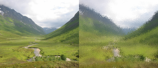
In this section some stranger filters are listed, these filters are not standard run of the mill image filters. But simple fun filters that fall into the category of area filters.
Pick an a random pixel within the sampling window.
Figure 5.8. jitter
-- a jittering filter implemented in lua

edge_duplicate=1 -- set edge wrap behavior to use nearest valid sample

function jitter(amount)
  local x,y
  var2=var1
  for y = 0, height-1 do
    for x = 0, width-1 do
      local nx,ny
      local r,g,b,a
      nx=x+(math.random()-0.5)*amount
      ny=y+(math.random()-0.5)*amount
      r,g,b,a=get_rgba(nx,ny)
      set_rgba(x,y, r,g,b,a)
    end
    progress(y/height)
  end
end

jitter(10)
Extend the convolve example, making it possible for it to accept a 7×7 matrix for it's values, add automatic summing to find the divisor and experiment with various sampling shapes.
Create a filter that returns the original pixel value if the variance of the entire sample window is larger than a provided value. How does this operation compare to kuwahara/snn?
[5] The despeckle filter for gimp is more advanced than a simple median filter, it also allows for being adaptive doing more work in areas that need more work, it can be set to work recursivly. For normal median operation adaptive and recursive should be switched off, the black level set to -1 and the white level to 256.