When creating tools to modify images, it is often vital to have an model of the image data. Using alternate ways to visualize the data often reveals other properties and/or enhances our ability to observe features.
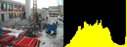
A histogram shows the distribution of low/high (dark/light) samples within an image.
The bars in the left portion of the histogram shows the amount of dark/shadow samples in the image, in the middle the mid-tones are shown and to the right the highlights.
A low contrast image will have a histogram concentrated around the middle. A dark image will have most of the histogram to the right, a bright image uses mostly the right hand side of the histogram, while a high contrast image will have few mid-tone values; making the histogram have an U shape.
The histogram in Figure 3.1, “histogram” spans from left to right, so it makes good use of the available contrast. The image is overexposed beyond repair, this can be seen from the clipping at the right hand (highlight side). This means details of the clouds in the sky are permantently lost.
Figure 3.1. histogram
-- utility function to set the RGB color for a rectangular region
function draw_rectangle(x0,y0,x1,y1,r,g,b)
  for y=y0,y1 do
    for x=x0,x1 do
      set_rgb (x,y, r,g,b)
    end
  end
end

function draw_histogram(bins)
  -- first we count the number of pixels belonging in each bin
  local bin = {}
  for i=0,bins do
    bin[i]=0
  end
  for y=0, height-1 do
    for x=0, width-1 do
      l,a,b = get_lab (x,y)
      bin[math.floor(bins * l/100)] = bin[math.floor(bins * l/100)] + 1
    end
    progress (y/height/2)
  end
  -- then we find the maximum number of samples in any bin
  max = 0
  for i=0,bins do
    if bin[i]>max then
      max=bin[i]
    end
  end
  -- and then plot the histogram over the original image.
  for i=0,bins do
    draw_rectangle((width/(bins+1))*i, height-(bin[i]/max*height),
             (width/(bins+1))*(i+1), height, 1, 1, 0)
    progress (i/bins/2+0.5)
  end
end

draw_rectangle(0,0,width,height,0,0,0)
draw_histogram(64)
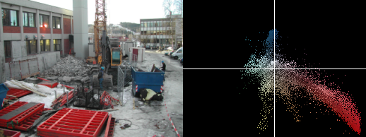
A chromaticity diagram tells us about the color distribution and saturation in an image. All pixels are plotted inside a color circle, distance to center gives saturation and angle to center specifies hue. If the white balance of an image is wrong it can most often be seen by a non centered chromaticity diagram.
![[Note]](images/note.png) | Origin in analog widget |
|---|---|
A chromaticity scope in the analog television world were traditionally created by conncting an oscilloscope to the color components of a video stream. This allowed debugging setting of the equipment handling the analog image data. |
Figure 3.2. chromaticity diagram
function draw_rectangle(x0,y0,x1,y1,r,g,b)
  for y=y0,y1 do for x=x0,x1 do set_rgb (x,y, r,g,b) end end
end

function draw_chromascope(scale)
  if width > height then
     scale = (scale * 100)/height
  else
     scale = (scale * 100)/width
  end
  for y=0, height-1 do
     for x=0, width-1 do
        l,a,b = get_lab (x,y)
        set_lab ( (a * scale) + width*0.5,
                  (b * scale) + height*0.5,
                   l,a,b)
     end
     progress (y/height)
  end
end

draw_rectangle(0,0,width,height,0,0,0)
draw_chromascope(4)
draw_rectangle(width*0.5,0,width*0.5,height,1,1,1)
draw_rectangle(0,height*0.5,width,height*0.5,1,1,1)
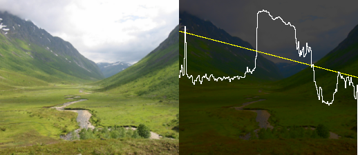
A luminiosity profile is the visualization of the luminance along a straight line in the image. The luminance plot allows a more direct way to inspect the values of an image than a histogram does.
In Figure 3.3, “luminance profile” the yellow curve indicates which line the profile is taken from, the brightness of the snow as well as the relative brightness of the sky compared to the mountains is quite apparent.
Figure 3.3. luminance profile
function draw_rectangle(x0,y0,x1,y1,r,g,b)
  for y=y0,y1 do for x=x0,x1 do set_rgb (x,y, r,g,b) end end
end

function lerp(v0,v1,r)
  return v0*(1.0-r)+v1*r
end

function draw_line(x0,y0,x1,y1,r,g,b)
  for t=0,1.0,0.001 do
    x = lerp(x0,x1,t)
    y = lerp(y0,y1,t)
    set_rgb (x,y,r,g,b)
  end
end

function lumniosity_profile(x0,y0,x1,y1)
  for y=0,height-1 do
    for x=0,width-1 do
       l,a,b = get_lab (x,y)
       set_lab (x,y, l*0.3,a,b)
    end
  end
  draw_line(x0,y0,x1,y1,1,1,0)
  prev_x, prev_y = -5, height*0.5
  for x=0,width do
     xsrc = lerp(x0,x1, x/width)
     ysrc = lerp(y0,y1, x/width)
     l,a,b = get_lab (xsrc,ysrc)
     y = height - (l/100) * height
     draw_line (prev_x, prev_y, x,y, 1,1,1)
     prev_x, prev_y = x, y
  end
end

lumniosity_profile(0,height*0.2, width,height*0.5)